Step 1: Load and Preview Data

If you have chemical mapping data on different RNA sequences, especially if they are not the same length, please separate data of each sequence into individual analyses.

As you can see in Step #3 and Step #4, you need to specify sequence information and annotate bands to match sequence. Thus, it only works for one input sequence.

In this tutorial, we will use the pfl riboswitch data to walk you through the HiTRACE pipeline. pfl riboswitch binds to ZMP (5-amino-4-imidazole carboxamide ribose-5′-monophosphate), and is described in detail by Trausch et al. 2015 and Ren et al. 2015. The data was originally collected in an RNA Puzzle blind modeling contest. Thus, it is a great example on how to analyze (new) data.

The collected 1D data contains conditions of nomod, SHAPE, DMS, CMCT, and all 4 ddNTP ladders. Data includes conditions of both in absence (minus) and in presence (plus) of the ligand. Each sample was run as both satuated (sat) and diluted (dil), which will be futher explained in Step #6. An overview of the 1D data is available here.

To load and preview data, we use the quick_look() command. It is a script that we use on daily basis to rapidly evaluate whether an experiment is successful. It also provides print-outs for keeping in notebooks.

First, let’s define the data directories and lane ordering:

filenames = { ...
    'pfl_1D_QC&CM_2015-05-02_1802', ...
    'pfl_1D_QC&CM_2015-05-02_1803', ...
    'pfl_1D_QC&CM_2015-05-02_1804', ...
    'pfl_1D_QC&CM_2015-05-02_1805', ...
};
ylimit = [2501, 6000];
reorder = [1:8, 17:64, 9, 13, 10, 14, 11, 15, 12, 16];

The ylimit variable defines the window of data time-series. When not specified (or as empty []), quick_look() can make a best guess of the relevant time window. Usually, we run with [] first. If the resulting auto-selected ylimit is unsatisfactory, we adujst it manually and rerun.

The reorder variable defines the display order of data lanes. When not specified (or as empty []), it follows the order of directories as defined in the filenames. Inside each directory, it sorts lanes according to a 96-wll plate layout by column, i.e. A01 - > B01 -> … -> G01 -> H01 -> A02 -> … -> H02 -> A03 -> … -> H12. Note that the indices in reorder should not exceed the total number of .ab1 files of all directories.

In this example, it reads in all ABI sequencer files (.ab1) from these 4 folders, crops to the time window, and reorders it in a way that the ddNTP ladder lanes are placed to the last. The names of .ab1 files is explicit on the data content.

Make sure you navigate to the working directory that contains the data directories (using cd dir_name).

We recommend keeping the well prefixes in each .ab1 filename. Please make sure that there is no well name collision between files within the same directory. Each directory should hold no more than 96 lanes.

Directory names should NOT end with a space. Otherwise it may cause ane error.

Now, you can run:

[d_align, d_ref_align, ylimit, labels] = quick_look(filenames, ylimit, reorder);

It reads in the data, subtracts a constant offset from all the profiles, and normalizes to the mean signal intensity. It returns the following variables:

You’ll see several windows that show steps along the automated read-in and first-pass alignment. Please DO NOT close figure windows before quick_look() finishes! Otherwise you may see an error about saving figures to .eps files.

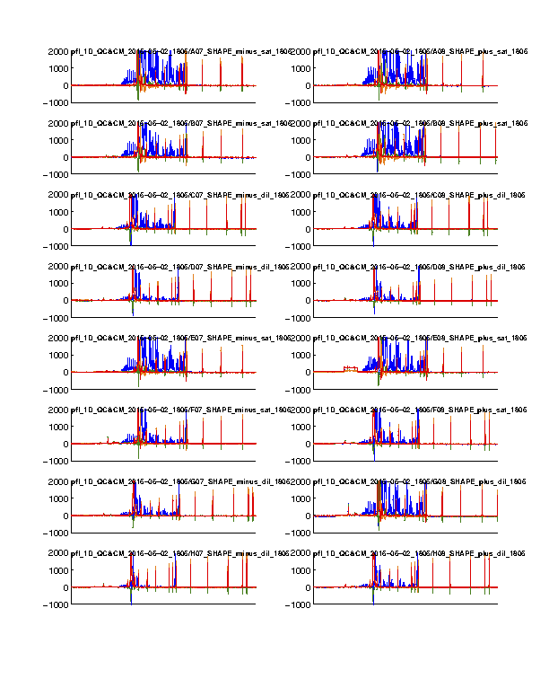
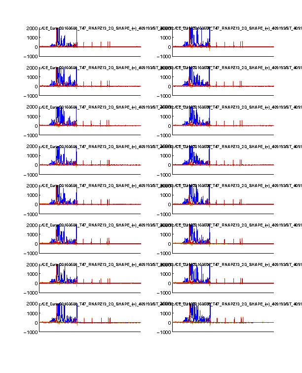
Figure 1: Time-series view of fluorescence profiles

The 4 channels are colored in blue, cyan, green, and red. Only the last 16 lanes are shown. In our standard setup, the signal channel (FAM) shows up in blue; and the reference channel (ROX) shows up in red.

The ROX channel should appear as digital spikes. The ssDNA sizes of ROX350 ladder used is described here.

The cyan and green channels should be mostly flat since we don’t typically load anything with these colors.

The FAM channel should have a lot of peaks, while the peaks should be reasonably tall in the plot. Most of the peaks in the middle should not be so tall that appear plateaued. A plateaued peak is due to the sensitivity ceiling of the fluorescence camera. The full-length extended band (right hand) is usally very strong and thus plateaued. This is why we run diluted data as well and correct for saturation in Step #6.

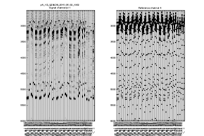
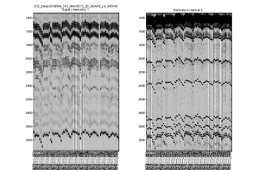
Figure 2: Raw traces

The signal channel and reference channel data are visualized as black/white heatmaps, side by side. These are raw data, as directly loaded from .ab1 files.

Check whether the ylimit is reasonable. None of the lanes should have their top or bottom truncated out.

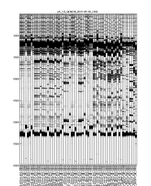
Figure 3: Intermediate traces after initial processing

The signal channel data visualized as heatmap. This is after profile alignment by groups, and intensity normalization.

Usually, any imperfections at this step should be fixed in Figure 4.

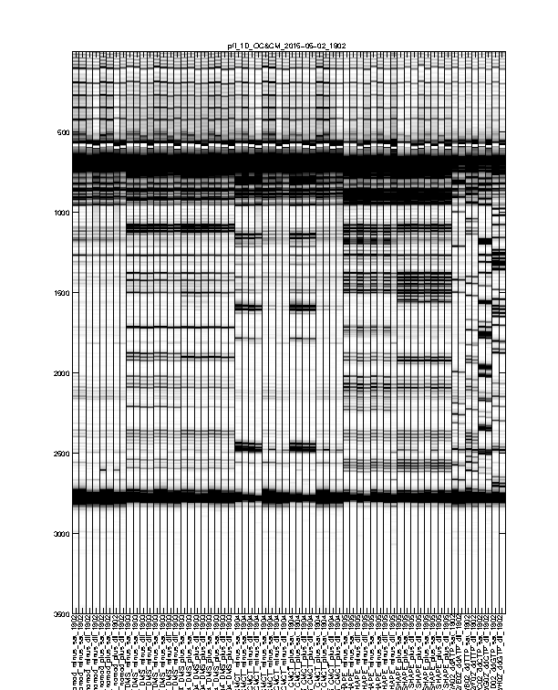
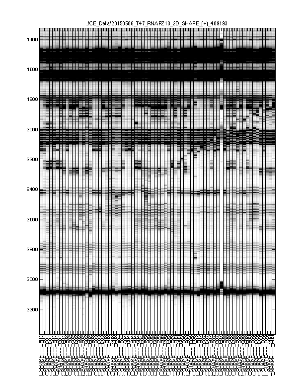
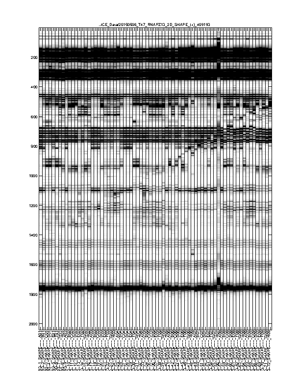
Figure 4: Final traces after further processing

The signal channel data visualized as heatmap. This is after baseline subtraction, piece-wise-linear alignment based on reference channel, and local alignment refinement.

This is the final trace that will carry on to downstream analysis. The alignment should be largely acceptable: the full-length extended band (bottom) should line up across all lanes since all samples are the same RNA. The lanes with similar property (e.g. same modifier) should have their signaure bands aligned to each other. The ddNTP ladders should be well-spaced, just like an old-fasion sequencing gel.

There could be some “waviness” across lanes of similar profiles. This is more obvious in Mutate-and-Map experiments. Step 2 takes care of such last refinement.

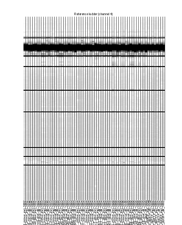
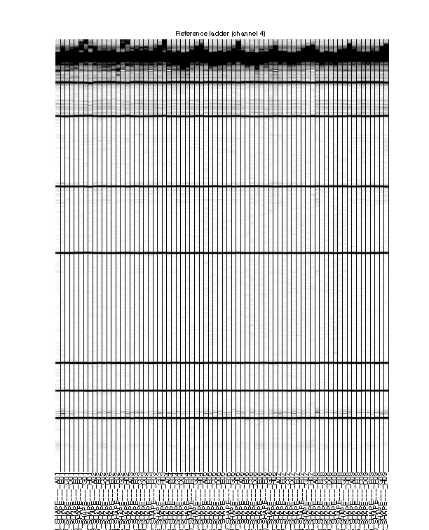
Figure 5: Final traces of reference channel

The reference channel data visualized as heatmap. This is after all processing, at the same stage as Figure 4. The reference channel is not used in any upcoming steps.

The ROX350 ladders should line up very well across all lanes

If you need to turn off the baseline subtraction or alignment, you can do so by changing the input to quick_look(). You can also apply leakage correction, or select other color channels to define which channel is the signal or which is the reference. For more information on command arguments and returns, please refer to help quick_look.

As an example of 2D data analysis, it is the same as 1D for this step.

filenames = {'pfl_2D_SHAPE_plus_409193'};
[d_align, d_ref_align, ylimit, labels] = quick_look(filenames, [], 1:72);

It is obvious that there is a bad lane showing no data in Figure 2. The pattern for that lane in Figure 3 and Figure 4 is an artifact/amplification of normalization. We will exclude this lane in the downstream analysis.

Troubleshooting

Certain common problems you may face:

• Final traces not aligned well.

So your Figure 4 looks more like the Figure 3 in the 1D example. Check your Figure 5:

If the reference channel is not aligned well, it could be the ylimit’s fault. Adjust the ylimit paying extra attention to the reference channel. Sometimes when certain lanes got cropped out of a ROX band, the alignment algorithm is confused by the mismatch of numbers of reference ladders. Enlarge your ymax and give it another try.

If no luck, check Figure 2 instead:

Although not aligned at all, all lanes should be roughly the same migration rate, i.e. the length of top to bottom of signals should be the same. If a lane is compressed or stretched (possibly due to buffer or voltage variations), quick_look() might not be able to rescue it.

• Error on saving figure.

Please close all windows and retry. Make sure you don’t switch between MATLAB windows, or close any figure windows while quick_look() is running. It saves the figures in the end, and a closed figure window will cause error.