Step 6: Data Corrections (for 1D data only)

For Mutate-and-Map data, we can draw inferences from the changes in the chemical mapping reactivities as mutations are carried out. Thus the relative values are OK. However, for quantitative analysis, we need to correct for several factors arise from the experiment measurements:

• Background Stops: the reverse transcriptase has intrinsic stops along the sequence. You may see such sites in a nomod profile. We need to subtract out these to estimate true chemical reactivities.

• Signal Attenuation: the reverse transcriptase terminates (is blocked) at the first modification site it encounters from the 3′ end. Thus, the number of cDNA fragments attenuates as the length gets longer. For a long RNA, it is easy to spot that the longer reverse transcription products will have attenuated intensity compared to shorter ones. We need to correct for such directional bias.

In principle, this could all be carried out accurately and analytically if we could measure the amount of unmodified product – the very longest (full-length extended )band in the capillary trace. But under ‘single hit conditions’, this fully extended band typically saturates our fluorescence detector. And this leads to the next item:

• Signal Saturation: the fluorescence camera of the CE machine has a certain detection range. For signals that are beyond the maximum value, they cannot be measured accurately and thus appear plateaued. This is common for the full-length extended band of the gel since the majority of input RNA are unmodified under single-hit kinetics. We dilute the same sample in order to retrieve the intensity of such peaks.

• Normalization: to scale up the final reactivity profile to a common standard so that reactivities from different experiment (e.g. different RNA) can be compared to each other. This is where we the GAGUA reference hairpin comes to help.

HiTRACE offers a likelihood-based framework for estimating the scaling and attenuation correction factors.

An obsolete script overmod_and_background_correct_logL() was used to optimize the attenuation coefficient (by a grid search) and the scaling for the background (by linear programming) so as to best match your expectation. Please use get_reactivities() instead!

We first need to define some parameters:

ref_segment = 'GAGUA';
ref_peak = get_ref_peak(sequence, ref_segment, offset);

It searches for GAGUA sequence (which is the pentaloop of both reference hairpins at 5′ and 3′) and records the indices of those residues into ref_peak.

Next, we define the standard deviation to use as a cutoff for saturation in unsaturate() step. We basically always use:

sd_cutoff = 1.5;

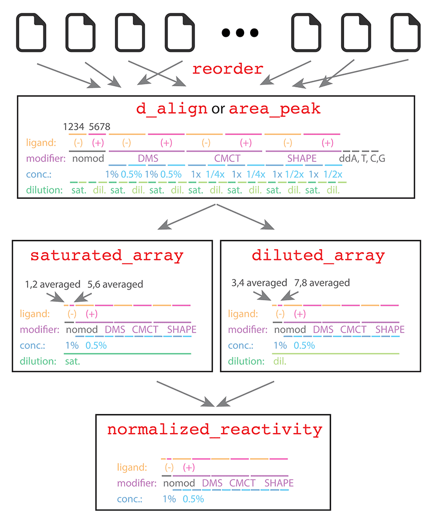
Now we need to split the dataset into a diluted half and a saturated (undiluted) half. We exclude any ddNTP lanes since we are not interested in quantitating them. For the DMS, CMCT, and SHAPE profiles, recall from the layout here. We know that:

saturated_idx = [9, 10, 13, 14, 17 ,18 ,21, 22, 25, 26, 29, 30, 33, 34, 37, 38, 41, 42, 45, 46, 49, 50, 53, 54];
diluted_idx = saturated_idx + 2;

Not to be confused with reorder from Step #1. The reordering of CE traces into our favorite ordering was done by quick_look(), and only needed once. From that moment on, the data in d_align (hence area_peak) is in the correct order. The indices in saturated_idx and diluted_idx should refer to area_peak locally.

For the nomod lanes, we need to average them before running get_reactivities(). Since conditions of absence and presence of ligand should not be mixed together, we do:

saturated_array_nomod = [mean(area_peak(:, 1:2), 2),  mean(area_peak(:, 5:6), 2)];
diluted_array_nomod = [mean(area_peak(:, 3:4), 2),  mean(area_peak(:, 7:8), 2)];

This is only needed for this example since it has replicates for each condition (e.g. 2 nomod lanes). Since we cannot subtract data to multiple background lanes, we are averaging them into 1 for each condition.

The above command averages lane 1 with 2 (without ligand), 5 with 6 (with ligand) for saturated nomod data; lane 3 with 4 (without ligand), 7 with 8 (with ligand) for diluted nomod data. Note the use of mean() by row. Now let’s merge the nomod data with all the other modifiers; same for errors:

saturated_array = [saturated_array_nomod, area_peak(:, saturated_idx)];
diluted_array = [diluted_array_nomod, area_peak(:, diluted_idx)];

saturated_error = [ ...
    mean(darea_peak(:, 1:2), 2), ...
    mean(darea_peak(:, 5:6), 2),...
    darea_peak(:, saturated_idx), ...
];
diluted_error = [ ...
    mean(darea_peak(:, 3:4), 2), ...
    mean(darea_peak(:, 7:8), 2),...
    darea_peak(:, diluted_idx), ...
];

The saturated_array should match saturated_error in column orders; same for diluted_array and diluted_error.

You can bypass the saturation correction if you did not perform dilution in your data. To do so, first still define your saturated_array as above. And then use diluted_array = saturated_array;. In this way, it won’t find anything to correct when comparing diluted_array to saturated_array.

Lastly, we need to specify the background columns for background subtraction. In our saturated_array has the columns as:

• nomod (-), nomod (+), DMS (-) x4, DMS (+) x4, CMCT (-) x4, CMCT (+) x4, SHAPE (-) x4, SHAPE (+) x4.

• [(-) and (+) mark ligand condition.]

All the (-) columns should be subtracted by nomod (-) while all the (+) columns should be subtracted by nomod (+). The column indices of nomod (-) and nomod (+) in saturated_array are 1 and 2, thus:

bkg_col  = [1, 2, 1, 1, 1, 1, 2, 2, 2, 2, 1, 1, 1, 1, 2, 2, 2, 2, 1, 1, 1, 1, 2, 2, 2, 2];

The numberings in bkg_col are based on column indices of saturated_array and diluted_array; not to be confused with saturated_idx and diluted_idx that are based on area_peak.

Finally, we can kick off the quantitation with:

[normalized_reactivity, normalized_error, seqpos_out] = get_reactivities( ...
    saturated_array, diluted_array, saturated_error, diluted_error, ...
    bkg_col, ref_peak, seqpos, [], data_types([1, 2, saturated_idx]), sequence, offset, sd_cutoff);

The argument data_types(saturated_idx) provides information of modifier identity for the lanes in saturated_array and diluted_array. Alternatively, data_types([1, 2, saturated_idx]) could be written as [{'nomod'}, {'nomod'}, data_types(saturated_idx)]. It’s important that it matches with the lanes identity in saturated_array and diluted_array, since area_peak is not used in this function call!

Recall the numbers of nucleotides reactive in GAGUA to DMS [2], CMCT [1], and SHAPE [5] are different. This information helps normalization step to scale up the profiles properly (by averaging among the right number of reactive nucleotides within GAGUA).

To better clarify the confusing indices and rearrangments, please read this illustration.

The run goes through the 4 processes, and waits you to continue between steps:

• Unsaturation

The saturated sample is on the left, diluted sample (after scaling up to match saturated sample) is in the middle, and the result after unsaturate() is on the right. The red lines show where a plateaued reactivity is found in saturated sample (by comparing to scaled diluted sample).

• Attenuation Correction

The data is now plotted by seqpos: 5′ on the top. The attenuation (lighter from bottom to top) is now corrected.

After this step, the extra full-length extened band is removed.

• Background Subtraction

After subtracting the background, the data now looks cleaner. Of course the _nomod_lanes are completely blank now.

• Normalization

Reactive residues in GAGUA reference loops are scaled to reactivity of 1.0 on average.

If no ref_peak is given, the normalized reactivites may have not been scaled correctly.

Once finished, the get_reactivities() command returns the following variables:

Again, you do not need to process your 2D dataset using this step!