Step 4: Sequence Assignment

Now we’re ready for the sequence assignment. The positions of the various bands are stored in a vector xsel. Let’s initiate it with empty []:

xsel = []; clf;

Only run this line at first time! It creates an empty xsel. If a variable named xsel already exists in the current workspace, its content will be erased. Do not run this line when you are revisiting this step!

clf clears a figure. It makes sure the interactive interface will inherit a full-size figure window.

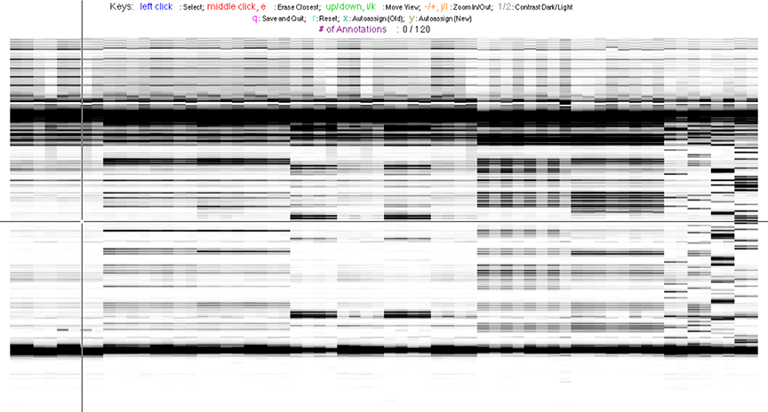
The goal is to specify the y-coordinates for each sequence position on the CE trace matrix, like the one showed in the overview.

Let’s start the interactive annotation. The core command is annotate_sequence. It brings up an interactive window, with your mouse as a crosshair.

[xsel, seqpos, area_pred] = annotate_sequence(d_align, xsel, sequence, offset, data_types, first_RT_nucleotide, structure);

Actions via keystrokes or mouse clicks are listed here:

Keys	Actions
left click	Add a sequence position to `xsel` at the y-coordinate clicked.
middle click, `e`	Erase the seqeuence position closest to where mouse clicked.
up/down, `i`/`k`	Move the view up or down.
`-`/`+`, `j`/`l`	Zoom in or out (vertically) of the view.
`1`/`2`	Adjust the display contrast darker or lighter.
`x`, `y`	Run auto-assign algorithm.
`r`	Reset all sequence positions, i.e. clear out `xsel` and start over.
`q`	Save `xsel` and quit interactive session.

More guides on how to operate:

Only when you hit q shall the result xsel be saved. So any action that causes error (e.g. closing the window) will abort the session, and leading to loss of unsaved xsel changes.

annotate_sequence() supports a mode that disables the “close window” button thus preventing from accidental close. To use it, call the command with the argument JUST_PLOT = 2. See help annotate_sequence for more details.

In JUST_PLOT = 2 mode, if error occurs and you want to close the disabled window, use command close_window().

Try not accidentally hit r, which will erase everything in xsel.
You may be switched to another MATLAB window when you type too fast. In such a case, use command + ` to switch back (Mac OS X).
The MATLAB mechanism behind this interactive session may result in inaccurate zoom-in on clicks. If you get ‘lost’, simply click q to save and quit. Then rerun the command to start over on the view.

Get started with some help!

Admittedly, this step is the most time-consuming (~~annoying~~) part of the entire HiTRACE pipeline. For starters, you may want to lend some help from the auto-assign algorithm that is aimed to do this for you. Although it does not get the job done perfectly, it is a good starting point that gonna save you a lot of time and trouble.

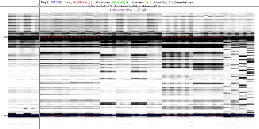
You only need to click 2 bands for it!

Click once at the top dark region (unextended primer) and
Click once at the bottom dark region (full-length extended band).

These 2 coordinates will be interpreted as the first and last band corresponding to your sequence. This helps the auto-assign algorithm in narrowing down the search space. Now hit x.

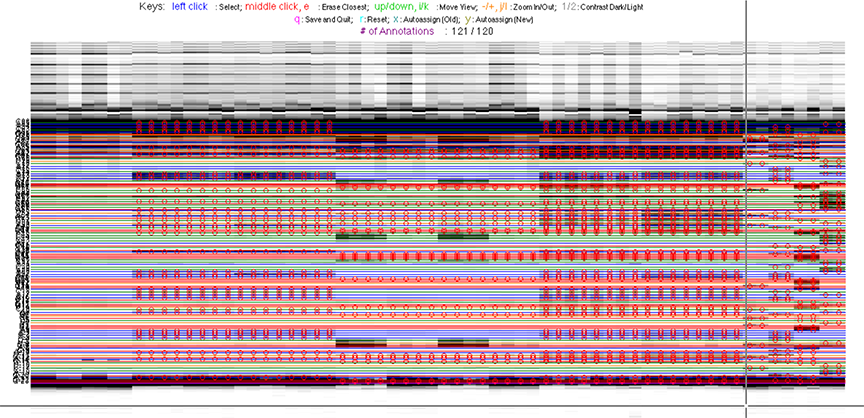
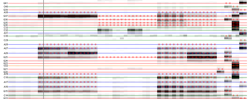
Once it finishes the calculation, you will see sequence positions filled out for you:

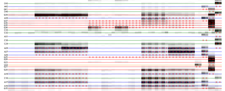
The horizontal lines are colored based on sequence identity (A, U, C, G). The red circles are where reactive bands are predicted to appear based on the combination of sequence, structure, and data_types. For example, an A residue that is unpaired is predicted to be reactive in a DMS experiment; while any residue that is base-paired is predicted to be unreactive in a SHAPE experiment. For ddNTPs ladder lanes, the circles correspond to sequence identity as in an old-fasion sequencing gel.

Note that there is a single-register shift between modifier profiles and ddNTPs profiles for the same nucleotide position. This is due to the nature of reverse transcription (RT): 1) RT stops BEFORE incorporation at the covalently modified nucleotide; 2) RT stops AFTER incorportaion of a ddNTP nucleotide.

Please remember that HiTRACE is aware of such single-register shift! It has shifted the numbers by 1 for you, so you only need to seek for a visual match between colors/circles and gel bands. If you read the labels on the figure carefully, you will find they are shifted by 1 from the circles.

Not done, yet …

As mentioned before, the auto-assign result need to be double checked before acceptance. Here are some guidelines on what to look out for:

Go over the sequence from the bottom upwards. Zoom in several times to space out bands for visual inspection. Adjust the contrast along the way as you move up.
There should be 1 extra band at the bottom. The extra band (appears magenta) is where the full-length extended product is. (See also the 121/120 caption in the figure top.)

Depending on where the modification is, RT can produce a cDNA whose length corresponds to the modified sequence position. Besides these S (length of sequence) products, there is one that corresponds to when no modification occurred, which is the full-length extended product. Under single-hit kinetic conditions, the majority of RNA transcripts are not modified. Thus, this bottom band is very strong.

We need to place a xsel band at the full-length extended band for attenuation correction in Step #6. It requires the intensity of this full-length extended band.

The horizontal line should go through the band at its center. When there is a discrepancy (or even disagreement) between your modification lanes and the ddNTP ladders, prioritize the positioning to the data you care.

Remember, the ddNTPs ladders are only used for assisting you in this step by tracking where the sequence goes. The band intensities of ddNTP ladders are not of interest for later quantitation.

The spacing between nucleotides should be even overall.

It is common that a region of consecutive G residues causes local compression. These bands may appear closer to each other than average.

Play with the contrast to reveal less obvious “hints” from the gel to help you locate. Since CE is gel-based, the spacing of the top (shorter fragments) portion of the traces is slightly larger.

Check if the reference hairpins are correctly assigned.

If you have the GAGUA reference hairpin at both ends (or either end) of your RNA transcript, they serve as good checkpoints for your sequence assignment.

All 5 residues of GAGUA are reactive to SHAPE; (only) both As are reactive to DMS; and only the U residue is reactive to CMCT.

Example of local shifts

Here are examples showing symptoms of incorrect sequence assignment.

Left: missing 1 band somewhere before this region causing guide circles to shift down.
Right: having 1 extra band somewhere before this region causing guide circles to shift up.

Once finished, the annotate_sequence() command returns the following variables:

Variable	Type	Description
`xsel`	1x(S+1) double	Band y-coordinates from the sequence assignment. Note that the command takes `xsel` as an argument, and updates it with your changes and returns it. S is the length of `sequence`.
`seqpos`	1x(S+1) int	Numbers of sequence positions from 5′ to 3′ end.
`area_pred`	SxN int	The predicted band positions, used for red circles drawing.

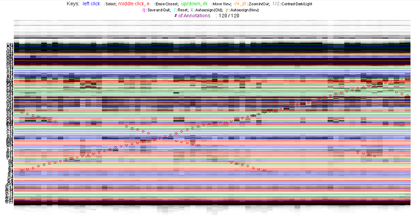
As an example of 2D data analysis, the commands are the same as 1D for this step. However, there is one difference:

Do NOT include the full-length extend band!

Yes, for 2D datasets, you should aim for 120/120, excluding the bottom full-length extra one. This is because:

In Mutate-and-Map data, we process it into Z_score as pseudo-free energy bonus instead of absolute reactivity. The calculation of Z_score is row by row (nucleotide by nucleotide), with the attenuation cancelled out. Thus, there is no need to include the full-length extended band for quantitation.

Because we are using number strings in data_types, the red circles mark where the predicted pertubation would show up based on structure and mutpos. It is obvious that these red circles form a main diagonal marking mutations (bottom left -> top right), as well as cross-diagonals marking helices based on given structure.