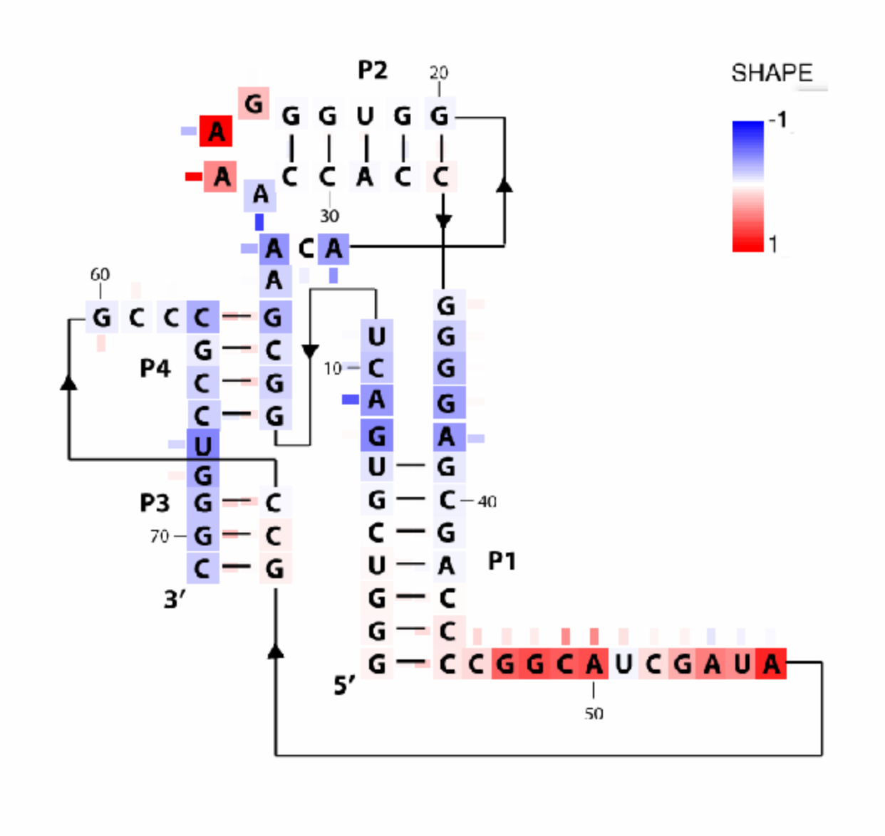
Color Secondary Structure Diagram
Congratulations! You’ve made it this far. It is usually helpful to plot the nucleotide-by-nucleotide reactivities onto a secondary structure diagram to investigate the structure of RNA. In this tutorial, you will learn how to plot colored reactivities boxes onto a secondary structure diagram in MATLAB using HiTRACE pipeline.
Example scripts and data used in this tutorial are included in the RiboPaint repository:
Preparations
-
Prepare TIFF Image
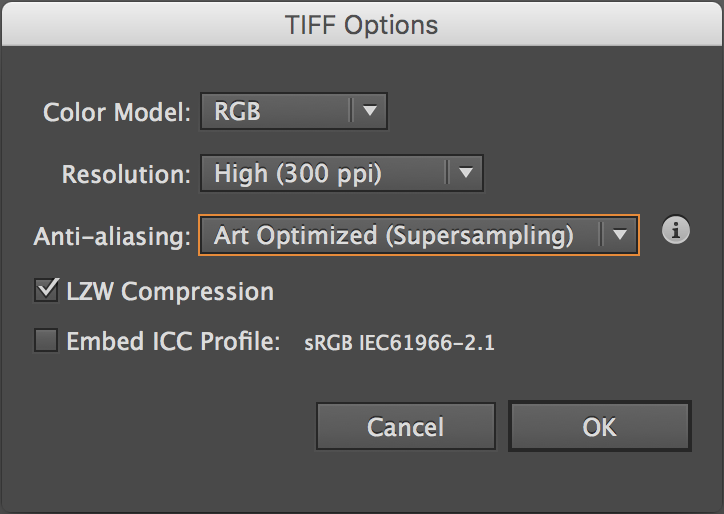
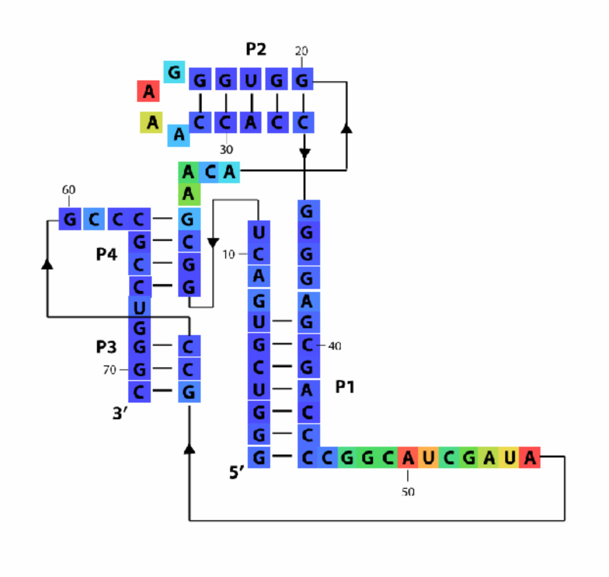
To make one of these diagrams, you’ll need a .tif file containing your secondary structure image. If you made your figure in Illustrator, export it as a .tif:
-
With RGB coloring (
CMYKcoloring will not work!) and LZW compression. -
Make sure to click “Use Artboards”
-
Prepare Reactivity Data
Reactivity data for each nucleotide position. Please make sure to trim the data to match the actual length and sequence to be plotted on the diagram. Excess 5′ and 3′ sequences should be discarded. Adjust the seqpos accordingly.
Now open MATLAB (don’t need to be from terminal).
d = load('pfl_1D.mat');

d_SHAPE_plus = d.d_SHAPE_plus(25:95);
d_SHAPE_minus = d.d_SHAPE_minus(25:95);

for i = [1:length(d.sequence)] - d.offset;
    if d.sequence(i + d.offset) == 'A' || d.sequence(i + d.offset) == 'C';
        d_DMS_CMCT_plus(i + d.offset) = d.d_DMS_plus(i);
        d_DMS_CMCT_minus(i + d.offset) = d.d_DMS_minus(i);
    else
        d_DMS_CMCT_plus(i + d.offset) = d.d_CMCT_plus(i);
        d_DMS_CMCT_minus(i + d.offset) = d.d_CMCT_minus(i);
    end;
end;
The above code loads the saved 1D analysis workspace into a variable called d. And trims SHAPE data into d_SHAPE_plus and d_SHAPE_minus. It combines DMS and CMCT data into d_DMS_CMCT_plus and d_DMS_CMCT_minus, respectively, based on sequence identity. In other words, it takes reactivity of A and C residues from DMS, reactivity of G and U resides from CMCT, and combine as one profile.
-
MATLAB Setup
We will load in the image file, click every base to set their locations, and then tell MATLAB to color these locations according to their reactivities. In this tutorial, we use the pfl riboswitch data to walk you through the HiTRACE pipeline.
First, we need to read in your image file. Make sure that you are in the same directory in MATLAB as the image file. Remember, it has to be .tif or .tiff.
mat_name = 'pfl_1D_color.mat';
imagex = imread('pfl_secstr.tif');
Now we have the image stored in pixel array named imagex, which is a HxWx3 uini8 matrix. The mat_name is the file we want to save our workspace to. We will be saving our work constantly. Now let’s set up some parameters:
residue_locations = [];
base_locations = [];
square_width = 28;

sequence = 'GGGUCGUGACUGGCGAACAGGUGGGAAACCACCGGGGAGCGACCCCGGCAUCGAUAGCCGCCCGCCUGGGC';
seqpos = 1:71;
offset = 0;
residue_locations and base_locations will contain the (X, Y) locations of each base - they tell MATLAB where to put colored boxes. square_width tells MATLAB how big to make the boxes.
Depending on your .tiff image size, the best value of
square_widthvaries. Try different values in the next step to see what size fits.
sequence, seqpos, and offset should match each other. Make sure all flanking sequences are removed (unless those are present in your diagram),
Interactive Annotation
-
Mark Box Coordinates
We need to mark the coordinates of each nucleotide on the image so that MATLAB can color them with boxes. We only need to do this once for each .tiff image and can reuse the coordinates for different paintings.
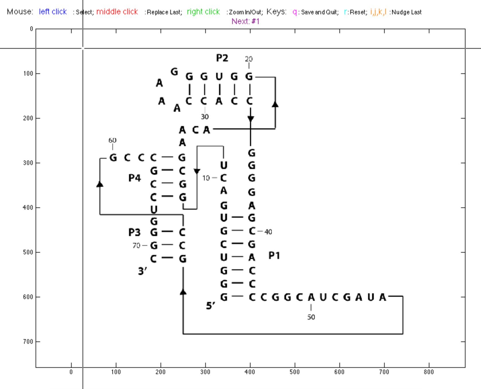
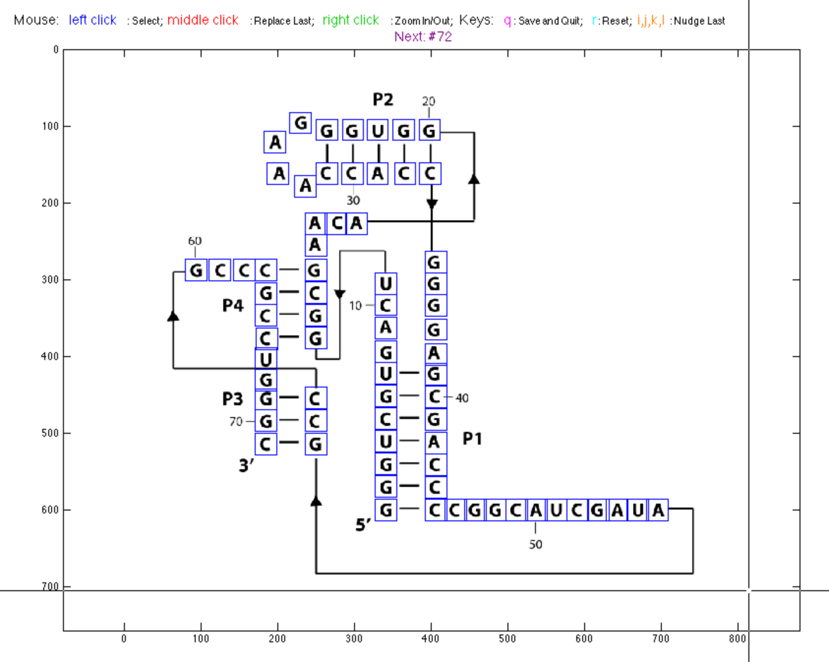
Let’s tell MATLAB where the bases are. pick_points() is an interactive scripts that load your image file, and place a box wherever you click. It is a similar experience to annotate_sequence() in Step #4. The colored boxes will go ‘behind’ the image (translucent), not covering letters or bonds.
residue_locations = pick_points(imagex, offset, residue_locations, square_width);
pick_points()supports a mode that disables the “close window” button thus preventing from accidental close. To use it, call the command with the argumentJUST_PLOT = 2. Seehelp pick_pointsfor more details.
In
JUST_PLOT = 2mode, if error occurs and you want to close the disabled window, use commandclose_window().
Use
JUST_PLOT = 1to show the boxes only, without invoking the interactive interface.
When started, it is empty. Use left click to place a box, middle click to erase a box. Remember, you can only remove the last box but not any one previous. Use right click to toggle zooming locally for better alignments.
Go through and click on each nucleotide to place a box around it. These boxes will represent SHAPE data. Be careful when clicking boxes: try you best to align the boxes of a helix. Currently, you need to do this by hand.
-
Mark Stub Coordinates
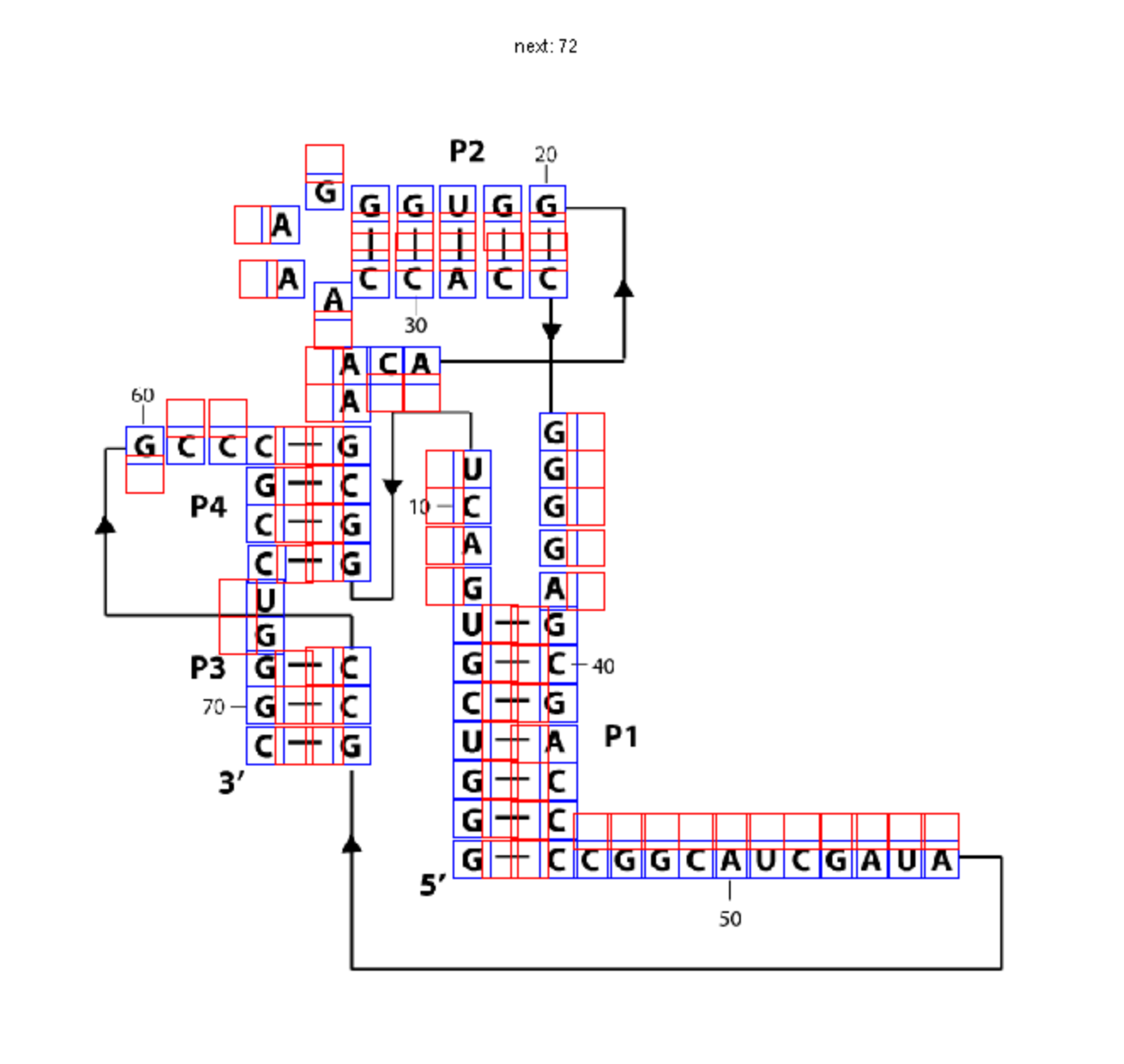
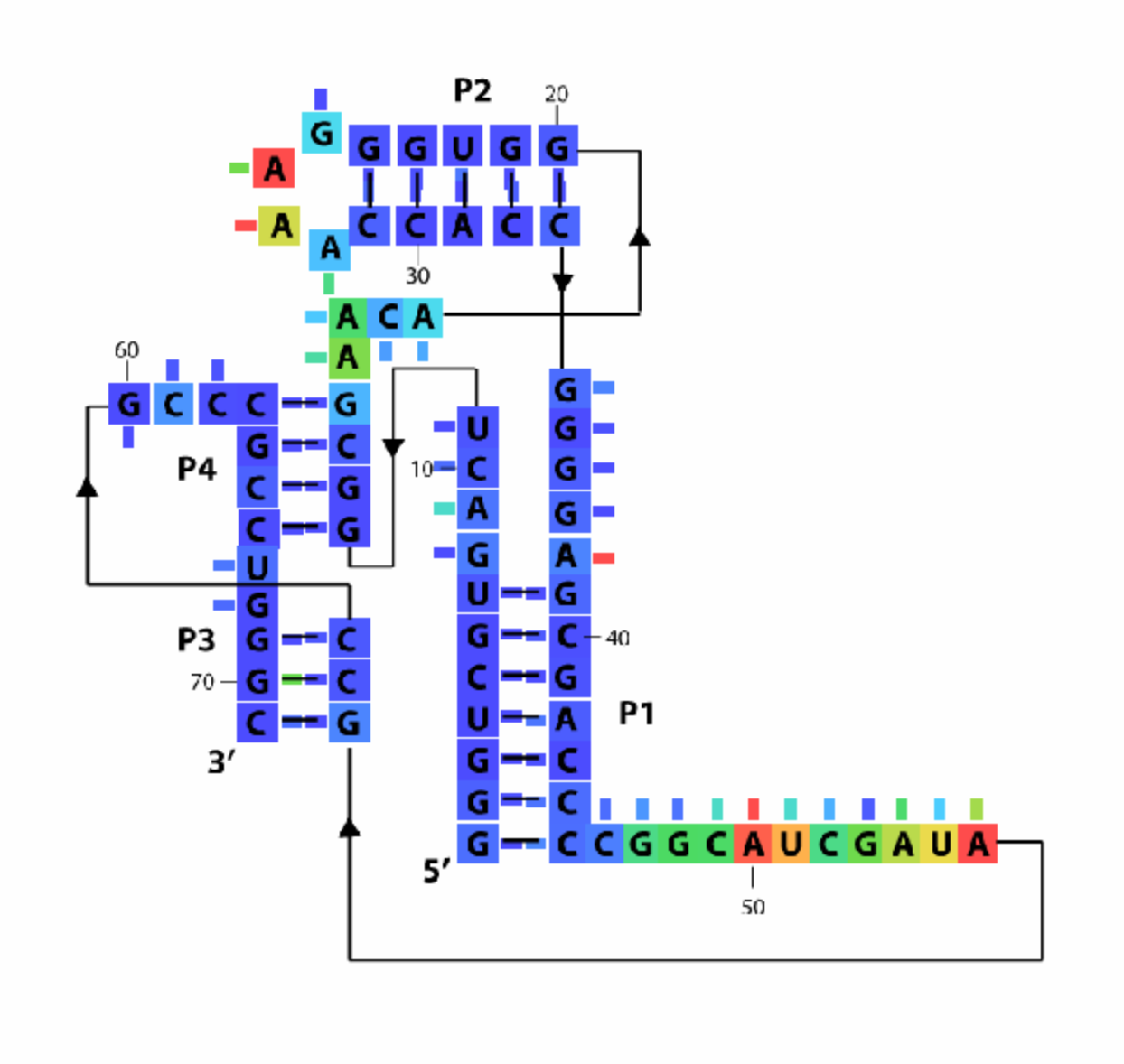
Next, we want to place ‘stubs’. These are used as ‘ticks’ pointing out from each nucleotide letter. They will be used to color the DMS/CMCT data. In this way, we can have both SHAPE and DMS/CMCT 1D data on the same graph.
Since the ‘stubs’ are right next to the letters (boxes), we use move_base_locations() to generate base_locations from residue_locations. This will make base_locations perfectly aligned to residue_locations in the final printout. For details, type help move_base_locations.
direction_cell = { ...
    [25, 29:33, 46:56, 61:62], ...          % top
    [18:24, 28, 60], ...                    % bottom
    [8:17, 26:27, 39:45, 57:59, 67:68], ... % left
    [1:7, 34:38, 63:66, 69:71], ...         % right
};
base_locations = move_base_locations(residue_locations, direction_cell, offset, square_width / 2, 5);
Relative locations of each residue of base_locations to residue_locations are specified by direction_cell, which is a 1x4 cell of double matrix. Each matrix tells the ensemble of residues whose base_locations is moved upward / downward / leftward / rightward from the corresponding (X, Y) coordinates of residue_locations.
You can manually type 3 out of 4 in
direction_celland usefill_direaction_cell()to fill the remaining one. Leaving the one with most elements to fill is always a good strategy. For details, typehelp fill_direction_cell. Double check thedirection_cellbefore running the next command. It will pop out WARNING if you missed any residue or typed one residue twice.
Place stubs for nucleotides in base pairs on the inside of the ‘bond’ between them, and stubs for unpaired nucleotides away from the stack. This allows you to compare your secondary structure with the data easily simply by reading down the stack.
An obsolete function
pick_bases()works the same way aspick_points()for this step. It is no longer used since clicking boxes is time-consuming.
You can still take advantage of pick_bases() to check if the base_locations are correct. Hit q to quit interactive window. Be careful to not accidentally click on the figure adding extra boxes!
base_locations = pick_bases(imagex, offset, residue_locations, base_locations, square_width);
Now save your work:
save(mat_name);
Painting
-
Get Color Scheme
First, tell MATLAB which box is which residue. whichres tells the order of reactivities in whattoplot. Please double-check that whichres should be an array starting with 1 and of same length with sequence. color_scheme controls what colors correspond to what values. Type help getcolor to see what values yield what colors. 17 is a rainbow (red-green-blue faded).
whichres = seqpos - offset;
color_scheme = 17;
Now let’s preview the color profile and make adjustments. whattoplot is the array containing reactivity values to be colored here.
whattoplot = d_SHAPE_plus;
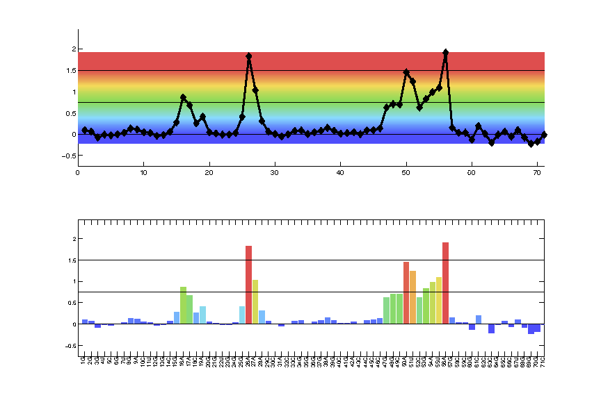
color_profile = color_palette(whattoplot, 1.5, 0, color_scheme, seqpos, sequence);
This will open a figure for a preview of coloring. Adjust the value 1.5 and 0 in the command to achieve optimal color ranges. The first value specifies the positive saturation value, and second specifies the negative saturation value; which are represented by black horizontal lines in the figure.
seqposandsequenceare optional for labeling the x-axis with residue names only. The coloring ranges is stored incolor_profilefor all future steps.
-
Color Boxes
Now let’s color the in-line boxes with:
imagex_1 = color_residues(imagex, residue_locations, whichres, whattoplot, color_profile, square_width);
This command will paint whattoplot onto the diagram at residue_locations with color settings specified by color_profile, with square_width boxes and stores new image in imagex_1.
-
Color Stubs
Now let’s color the out-line stubs! Note that this command takes the previous, SHAPE-colored diagram imagex_1 as the first parameter (instead of imagex).
whattoplot = d_DMS_CMCT_plus;
color_profile = color_palette(whattoplot, 1.5, 0, colorscheme, seqpos, sequence);
imagex_2 = color_bases(imagex_1, base_locations, residue_locations, whichres, whattoplot, color_profile, square_width / 2);
-
Add Legend
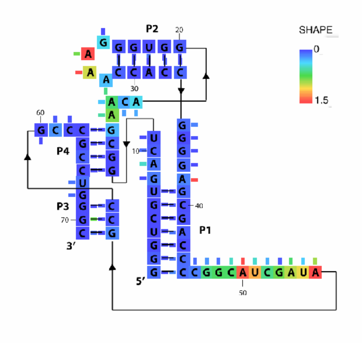
The last step is to paint a legend of color ranges on the diagram. Everything with the legend can be handled by defaults if you don’t feel like messing with it. Just run:
imagex_3 = color_legend(imagex_2, color_profile, square_width);
For pros, let’s setup the following parameters first:
orient_legend = [1 0];
pos_legend = [1 3 5 4];
labels = {'1.5', '0', 'SHAPE  '};
font_size = 0.8;
orient_legendprovides the orientation of legend bar. It consists of two 0 or 1 numbers: 1st one tells horizontal legend (0) or vertical legend (1); 2nd one tells the color gradient direction.
pos_legendtells the position and size of the legend. It consists of 4 numbers: 1st one tells which corner of the diagram should the legend be located, top-left (0) or top-right (1) or bottom-left (2) or bottom-right (3); 2nd one tells the distance between legend and nearest horizontal border; 3rd one tells the distance between legend and neatest vertical border; 4th one tells the size (length) of legend. Width of legend will always be 1; 2nd, 3rd and 4th number here are in unit ofsquare_width.
labelstells the labels to place on the legend. It consists of 3 strings: 1st one tells the label for positive saturation value; 2nd one tells the label for negative saturation value; 3rd one tells the title of legend.
font_sizetells the size of labels, in unit ofsquare_width. For details, typehelp color_legend.
Put the whole thing together, now! Note that this command takes the previous, DMS/CMCT-colored diagram imagex_2 as the first parameter.
imagex_3 = color_legend(imagex_2, color_profile, square_width, orient_legend, pos_legend, labels, font_size);
If the
color_legend()encounters error, just skip this step. You can add the legend in other ways, e.g. Illustrator. The rasterized text used incolor_legend()may cause problem sometimes.
You can paint multiple legends if different color ranges are used.
Plus, there is no need to paint the boxes following the order here: paint the stubs only, paint the boxes only, or paint the stubs first are fine.
-
Output Diagram
Finally, let’s save the image back to a .tif file by:
image_output(imagex_3, 'pfl_secstr_color_plus', 300);
save(mat_name);
This will save imagex_3 to the filename given here, with resolution 300 dpi.
More Fun
Since we have spent so much time on pick_points(), let’s make more diagrams with no effort:
whattoplot = d_SHAPE_minus;
color_profile = color_palette(whattoplot, 1.5, 0, color_scheme, seqpos, sequence);
imagex_1 = color_residues(imagex, residue_locations, whichres, whattoplot, color_profile, square_width);

whattoplot = d_DMS_CMCT_minus;
color_profile = color_palette(whattoplot, 1.5, 0, color_scheme, seqpos, sequence);
imagex_2 = color_bases(imagex_1, base_locations, residue_locations, whichres, whattoplot, color_profile, square_width/2);

imagex_3 = color_legend(imagex_2, color_profile, square_width, orient_legend, pos_legend, labels, font_size);
image_output(imagex_3, 'pfl_secstr_color_minus', 300);
The above code does the same thing for (-) ligand data. We can also plot the difference between (-) and (+) conditions. In this case, we choose a different color_scheme that is blue-white-red (faded).
color_scheme = 1;

whattoplot = d_SHAPE_plus - d_SHAPE_minus;
color_profile = color_palette(whattoplot, 1, -1, color_scheme, seqpos, sequence);
imagex_1 = color_residues(imagex, residue_locations, whichres, whattoplot, color_profile, square_width);

whattoplot = d_DMS_CMCT_plus - d_DMS_CMCT_minus;
color_profile = color_palette(whattoplot, 1, -1, color_scheme, seqpos, sequence);
imagex_2 = color_bases(imagex_1, base_locations, residue_locations, whichres, whattoplot, color_profile, square_width/2);

labels = {'1', '-1', 'SHAPE  '};
imagex_3 = color_legend(imagex_2, color_profile, square_width, orient_legend, pos_legend, labels, font_size);
image_output(imagex_3, 'pfl_secstr_color_diff', 300);
save(mat_name);
Bonus: Vectorized Figures
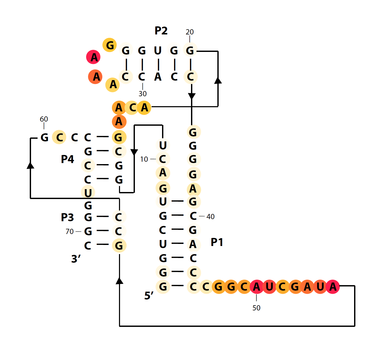
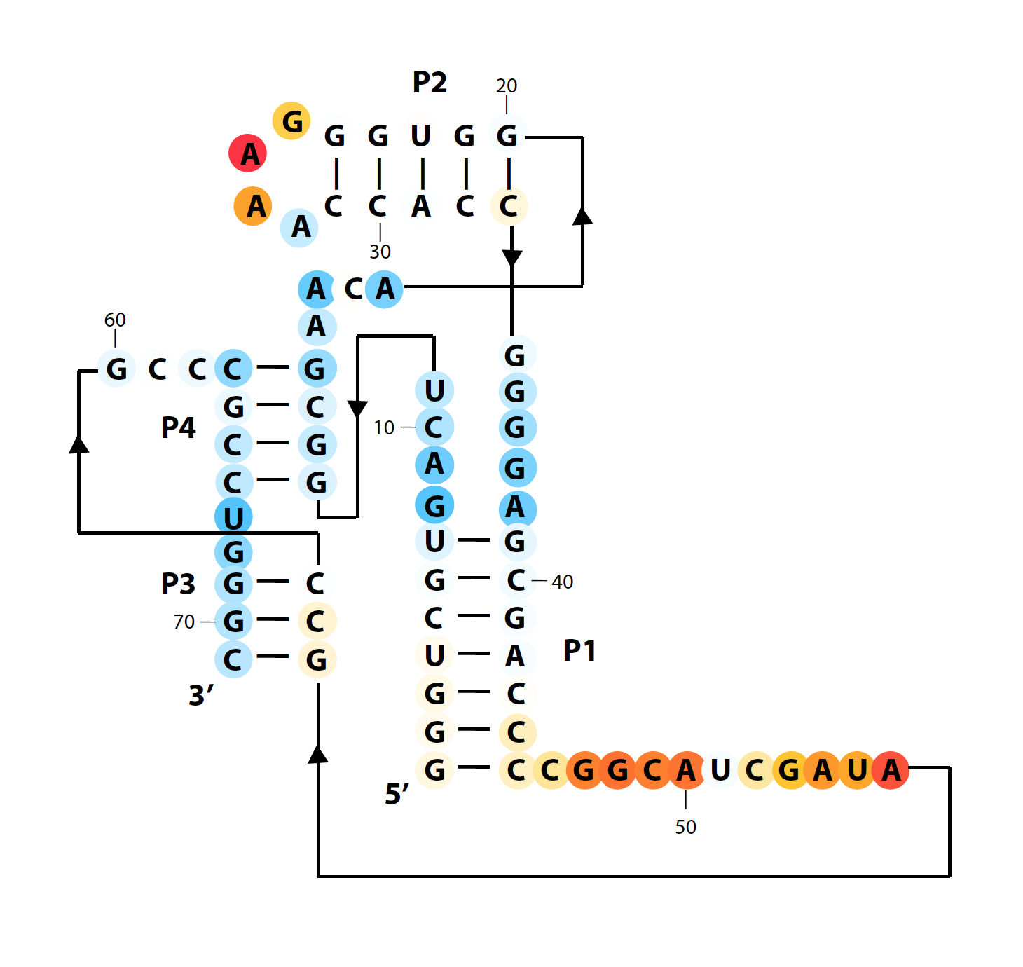
The previous .tiff files are rasterized with fixed resolution (300 dpi). We created a variant function that produces vectorized color diagrams. It is in same style with VARNA (white-orange-red circles, not squares).
color_scheme = 12   % publication-use red-yellow-white
whattoplot = d_SHAPE_plus;
color_profile = color_palette(whattoplot, 1.5, 0, color_scheme, seqpos, sequence);

color_circles(imagex, residue_locations, whichres, whattoplot, color_profile, square_width, 'circ_SHAPE_plus');
You can set the
is_roundargument back inpick_points()for circles (on display). Thecolor_residues()command also supports argumentis_circle, but its output is always rasterized TIFF matrix.
Same for difference plots:
color_scheme = 13   % publication-use red-white-blue
whattoplot = d_SHAPE_plus - d_SHAPE_minus;
color_profile = color_palette(whattoplot, 1, -1, color_scheme, seqpos, sequence);

color_circles(imagex, residue_locations, whichres, whattoplot, color_profile, square_width, 'circ_SHAPE_diff');
The circles are written to a .eps file named after the last argument in color_circles(). Now you can open the .eps file in Illustrator, copy over all the circles into your original diagram file, place them in the back, and resize (keep aspect-ratio) to match.
The final results are here: (+) SHAPE, and diff:
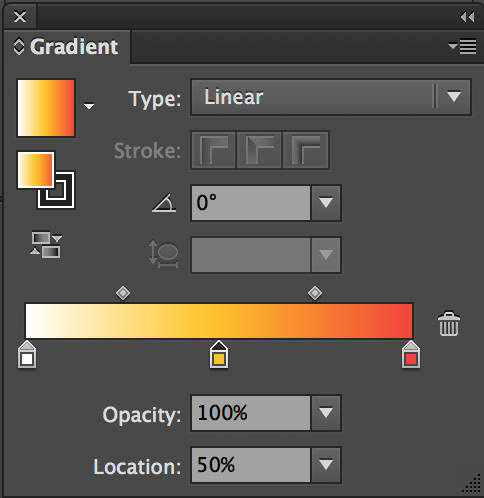
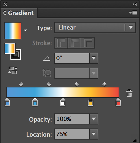
Since we are using Illustrator, you can add a legend with text showing the gradient:
For
color_scheme = 12, use gradient: 0%#ffffff, 50%#ffc107, and 100%#f44336.
For
color_scheme = 13, use gradient: 0%#5496d7, 25%#03a9f4, 50%#ffffff, 75%#ffc107, and 100%#f44336.
