Step 12: Visualize Secondary Structure (optional)
This step requires proper setup of the package biers. Please follow the installation guides there. Note that this step only requires the Biers and VARNA part.
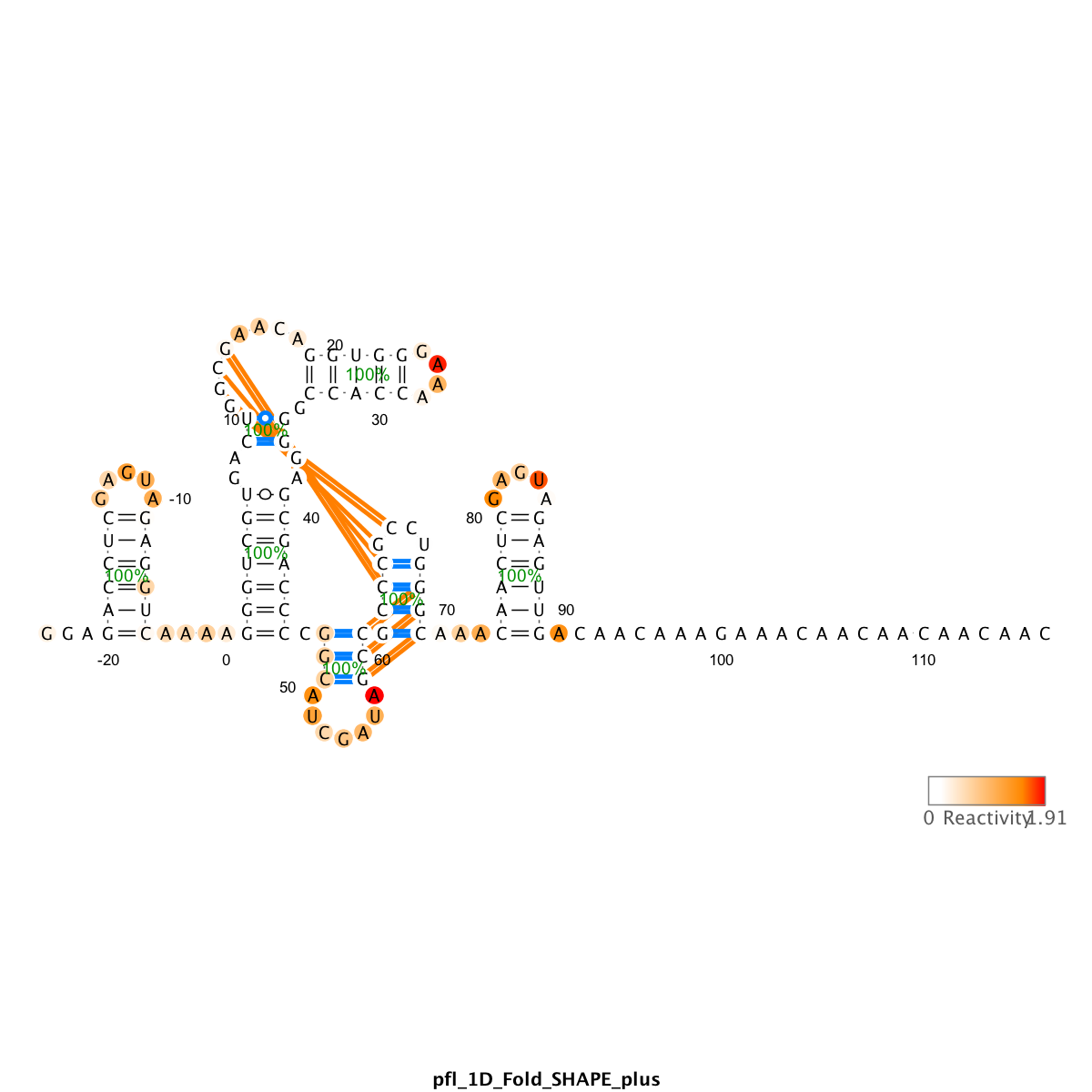
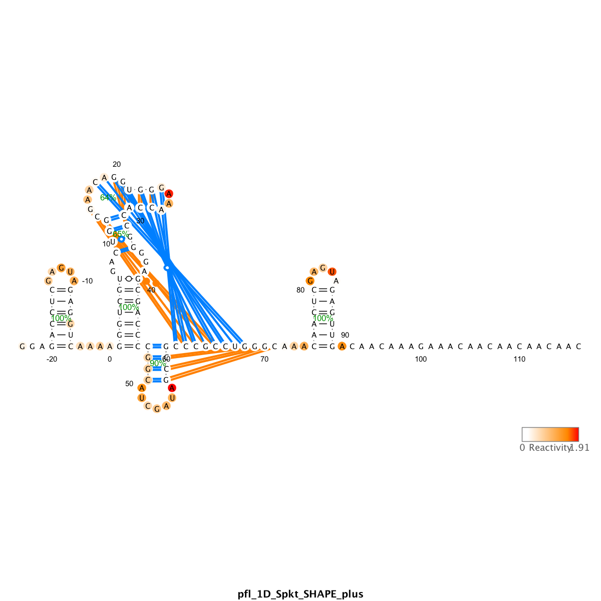
We use the output_varna() command to render files that utilize the VARNA applet. It draws the RNA sequence into the secondary structure, with nucleotides colored with their reactivity values, and shows helix-wise confidence estimate based on bootstrap bpp.
output_varna('pfl_NA', sequence, structure_NA, structure, structure_NA, offset, [], [], [], bpp_NA);
In the above code, the structure_NA, which is the result of the prediction run, is used as display. It also compares between structure (reference structure that has been used in sequence assignment) with structure_NA and draw the differences in lines.
Since this run was using no data (thus no bootstrap), the values in
bpp_NAare all 100%, and are not informative.
We can create ** pages for all the runs we have in Step 11:
output_varna('pfl_1D_Fold_SHAPE_minus', sequence, structure_1D_Fold_SHAPE_minus, structure, structure_1D_Fold_SHAPE_minus, offset, [], [], [d_SHAPE_minus; zeros(20, 1)], bpp_1D_Fold_SHAPE_minus);
output_varna('pfl_1D_Spkt_SHAPE_minus', sequence, structure_1D_Spkt_SHAPE_minus, structure, structure_1D_Spkt_SHAPE_minus, offset, [], [], [d_SHAPE_minus; zeros(20, 1)], bpp_1D_Spkt_SHAPE_minus);

output_varna('pfl_1D_Fold_SHAPE_plus', sequence, structure_1D_Fold_SHAPE_plus, structure, structure_1D_Fold_SHAPE_plus, offset, [], [], [d_SHAPE_plus; zeros(20, 1)], bpp_1D_Fold_SHAPE_plus);
output_varna('pfl_1D_Spkt_SHAPE_plus', sequence, structure_1D_Spkt_SHAPE_plus, structure, structure_1D_Spkt_SHAPE_plus, offset, [], [], [d_SHAPE_plus; zeros(20, 1)], bpp_1D_Spkt_SHAPE_plus);

output_varna('pfl_2D_Fold_SHAPE', sequence, structure_2D_Fold_SHAPE, structure, structure_2D_Fold_SHAPE, offset, [], [], [], bpp_2D_Fold_SHAPE);
output_varna('pfl_2D_Spkt_SHAPE', sequence, structure_2D_Spkt_SHAPE, structure, structure_2D_Spkt_SHAPE, offset, [], [], [], bpp_2D_Spkt_SHAPE);
For example, the blue lines are helices that are predicted by RNAstructure using data, but are not present in the reference structure (false positive). The orange lines are false negative, i.e. helices not captured by prediction.
Right click on the VARNA applet to bring out the menu. You can change the drawing algorithm, rotate the graph, and other functions. Save to .png or .eps files for future use. .eps is vectorized and more suitable for publications.
To interpret the predictions,
- Compare to the prediction with no data.
You want to know how much your data influences the secondary structure prediction. The best way is to compare to the prediction with no data.
- Visual check for reactivity agreement.
Are predicted helices protected/unreactive? Are predicted loops/single-stranded regions reactive?
Are the GAGUA reference hairpins predicted correctly?
- Pseudoknot
The ShapeKnot algorithm only allows one pseudoknot to be predicted. If your reference structure has more than 1, it cannot capture all.
You can use the reference structure as display structure to read out if any of the bootstrapping runs captured the missing pseudoknot. Or you can plot the
bpp.
When it fails to capture a pseudoknot, it usually makes up some other local helix instead. This is obvious that the made-up helix usually looks odd: reactive stems and/or protected loops.
- Bootstrap values
The higher the helix-wise confidence, the more robust the prediction. Usually > 90% is very good. Pseudoknots, if captured, still tend to have lower bootstrap numbers.
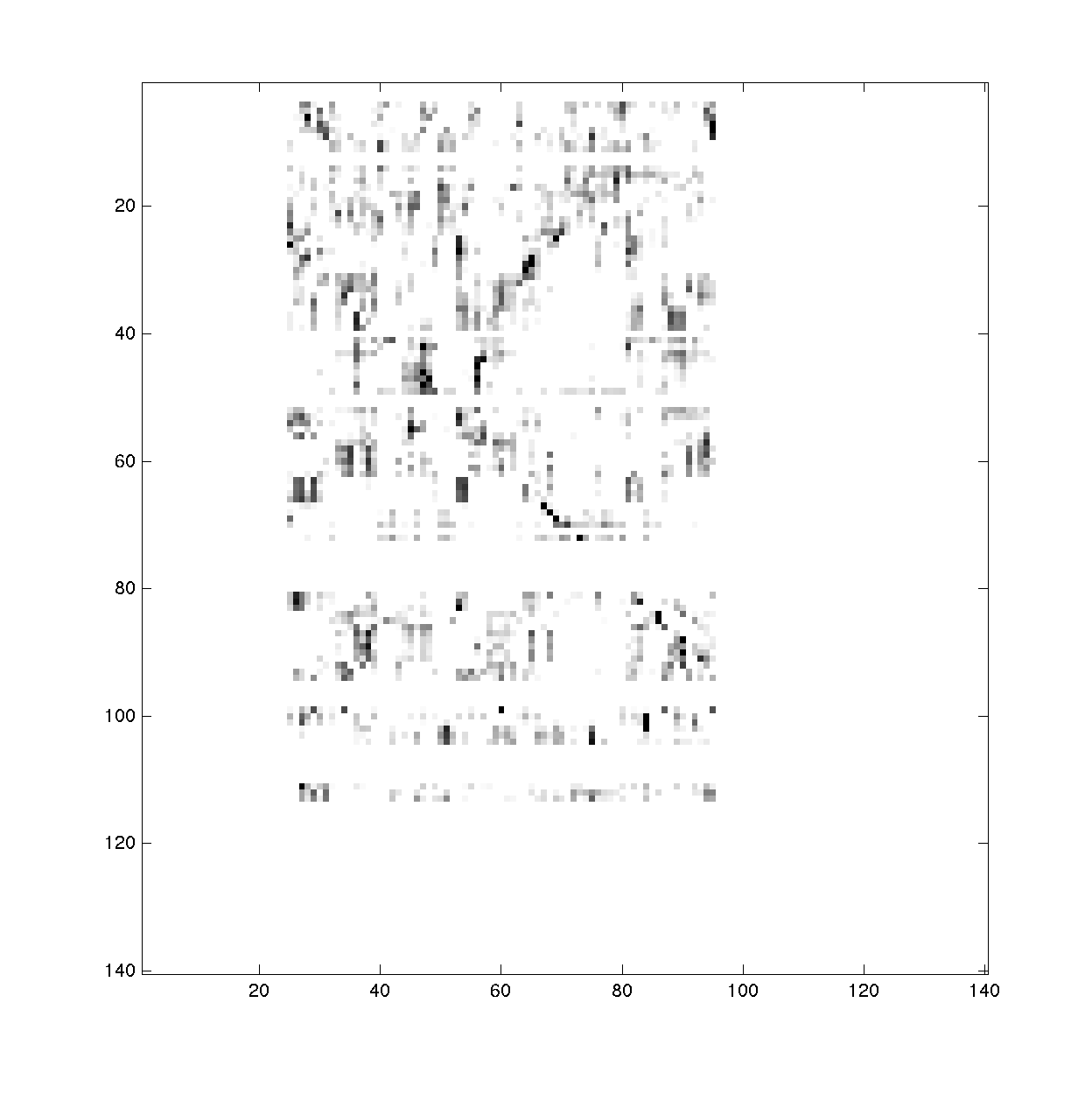
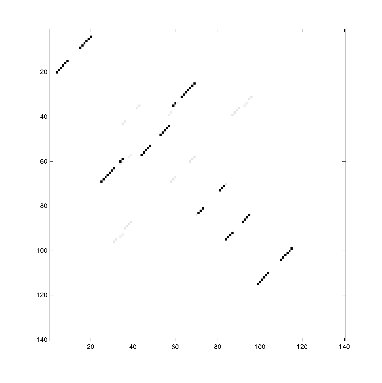
To visualize the bpp, we use the print_bpp_Z() command:
print_bpp_Z(bpp_2D_cutoff_mean, Z_cutoff_mean, -15, '2D_cutoff_mean');
This command generates images of the bpp and Z. It asks for a scaling factor for the Z-score figure.
- Previous: Predict secondary structure
- Back: Biers
- Back: HiTRACE


