Step 7: Error Estimates (for 1D data only)

For or 1D reactivity data, since there are replicates for each modifier profile, we would recommend checking consistency of those first. The first 8 lanes after 2 nomod are DMS, and we can plot those 4 (-) ligand lanes together with:

plot(normalized_reactivity(:, 3:6))

HiTRACE offers the function average_data_filter_outliers(), which takes traces and initial error estimates; figures out outlier points and even outlier traces; and then returns reasonable final values and error estimates:

[d_DMS_minus, da_DMS_minus, flags] = average_data_filter_outliers( ...
    normalized_reactivity(:, 3:6), normalized_error(:, 3:6), [], seqpos_out, sequence, offset); 

This step only concerns error estimates across replicates. If your experiment only involves one lane for each condition, you do not need to run this command. And use normalized_error directly instead.

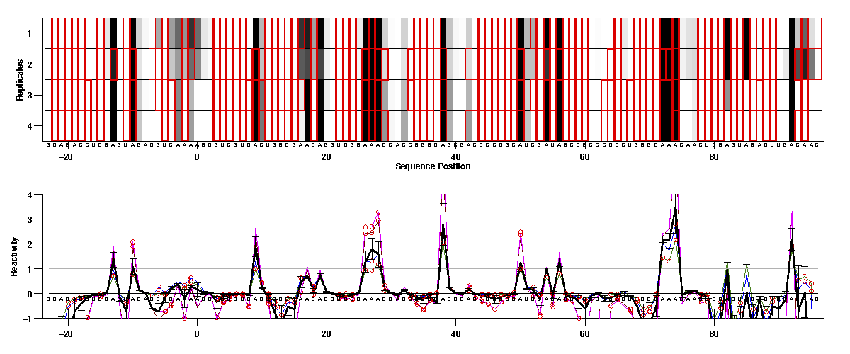
We can see the first 2 (blue & green) are in good agreement; so are the last 2 (red & magenta). But they do not agree with each other. In our experiment, 2 different modifier concentration were tried. And in this case, we think the first condition (e.g. DMS 1.0%) is better.

[d_DMS_minus, da_DMS_minus, flags] = average_data_filter_outliers( ...
    normalized_reactivity(:, 3:4), normalized_error(:, 3:4), [], seqpos_out, sequence, offset); 
[d_DMS_plus, da_DMS_plus, flags] = average_data_filter_outliers( ...
    normalized_reactivity(:, 7:8), normalized_error(:, 7:8), [], seqpos_out, sequence, offset); 

[d_CMCT_minus, da_CMCT_minus, flags] = average_data_filter_outliers( ...
    normalized_reactivity(:, 11:12), normalized_error(:, 11:12), [], seqpos_out, sequence, offset); 
[d_CMCT_plus, da_CMCT_plus, flags] = average_data_filter_outliers( ...
    normalized_reactivity(:, 15:16), normalized_error(:, 15:16), [], seqpos_out, sequence, offset); 

[d_SHAPE_minus, da_SHAPE_minus, flags] = average_data_filter_outliers( ...
    normalized_reactivity(:, 19:20), normalized_error(:, 19:20), [], seqpos_out, sequence, offset); 
[d_SHAPE_plus, da_SHAPE_plus, flags] = average_data_filter_outliers( ...
    normalized_reactivity(:, 23:24), normalized_error(:, 23:24), [], seqpos_out, sequence, offset); 

For simplicity, we created variables (e.g. d_DMS_minus) to hold individual reactivity values. We can now make a figure and evaluate the data (see Step #7).

Here are some checkpoints to go over:

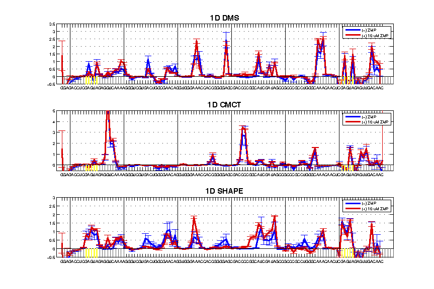
• GAGUA Reference Loops Reactivity: the nubmer of reactive nucleotides should meet the expectation based on the modifier. Also, it tests whether the GAGUA pentaloop is formed properly.

The 1D example has good GAGUA pentaloops, see the SHAPE profile for 5 reactive nucleotides and protected stems flanking the GAGUA. If the profile looks different, it may be your flanking sequence interferes with proper folding by interacting with the region of interest.

• Attenuation: the reactivity profile should be corrected for it. A good indicator is to compare the GAGUA reference loops of both ends. They should be the same ‘height’ in the plot.

The 1D example here has attenuation issues. The CMCT profile is generally bad, while the DMS is still attenuation biased, and the SHAPE profile is better but not perfect.

• Negative Values: negative values are resulted from background subtraction where the nomod trace has higher value than modifier. This is usually a result of strong reverse transcriptase stops.

Trace back where the negative values are. If there is a strong nomod background, it might be excusable. It could be due to degradation, or RNA activity (e.g. self-cleavage). A consecutive region of negative numbers ‘flying-off’ is a red flag. Slightly negative values (< 0.1) are no need to worry.