Step 5: Peak Fitting

Since we have done the hard work assigning where each band is, it is time to collapse the area of each peak into one intensity reading. To do so, we run it with one command:

[area_peak, darea_peak] = fit_to_gaussians(d_align, xsel);

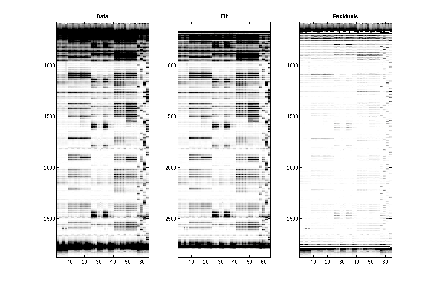
It takes the d_align traces and the band positions in xsel, and fits electrophoretic traces to sums of Gaussians. It produces a figure:

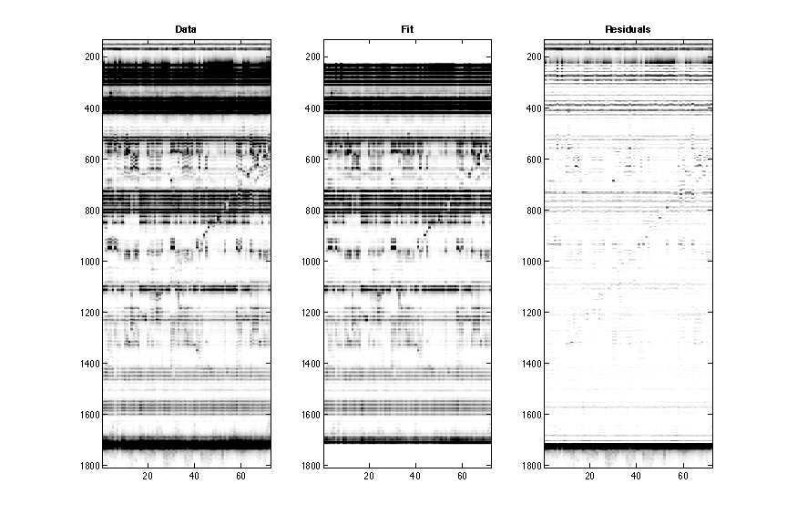
You’ll see the original data on the left, the fitted profiles in the middle, and residuals on the right. There is often a lot of noise (alternating black and white bars) at the top and bottom of the plot; the very large signals there are often saturated and not reproduced well by Gaussians. [That’s OK, we’ll ignore that data later.]

Most of the traces should be captured in the middle. Some minor leaks would fall to the right, and it is fine. The regions outside of our annotate region are not captured.

Note that this fit does not try to optimize the Gaussian widths (its assumed to be 0.25 times the mean peak spacing) or the band positions. To do that more complex fit, you can use do_the_fit(). But watch out since this can lead to spurious fluctuations especially for nearly merged bands.

Once finished, the fit_to_gaussians() command returns the following variables:

As an example of 2D data analysis, the commands are the same as 1D for this step.

[area_peak, darea_peak] = fit_to_gaussians(d_align, xsel);
area_peak(:, 56) = 0;
darea_peak(:, 56) = 0;

We erase lane 56 since it was bad data. This is to prevent accidental interpretation.